CurveSimilarities documentation

A collection of curve similarity measures.

There are tons of similar packages published on PyPI, but this one aims to be the most NumPy-friendly and the easiest to use.

API reference

To reproduce the examples, run the following code first:

import numpy as np
from curvesimilarities import *
from curvesimilarities.util import *

Warning

The similarity functions do not sanitize the vertices of input polygonal curves. Make sure your curves do not have consecutive duplicate vertices.

Fréchet distance

Continuous and discrete Fréchet distances.

curvesimilarities.frechet.fd(P, Q, rel_tol=0.0, abs_tol=2.220446049250313e-16)

(Continuous) Fréchet distance between two open polylines.

Let \(f: [0, 1] \to \Omega\) and \(g: [0, 1] \to \Omega\) be curves in a metric space \(\Omega\). The Fréchet distance between \(f\) and \(g\) is defined as

\[\inf_{\alpha, \beta} \max_{t \in [0, 1]} \lVert f(\alpha(t)) - g(\beta(t)) \rVert,\]

where \(\alpha, \beta: [0, 1] \to [0, 1]\) are continuous non-decreasing surjections and \(\lVert \cdot \rVert\) is the underlying metric. The Euclidean metric is used in this function.

Parameters:

Pndarray

A \(p\) by \(n\) array of \(p\) vertices of a polyline in an \(n\)-dimensional space.

Qndarray

A \(q\) by \(n\) array of \(q\) vertices of a polyline in an \(n\)-dimensional space.

rel_tol, abs_toldouble

Relative and absolute tolerances for parametric search of the Fréchet distance.

Returns:

distdouble

The (continuous) Fréchet distance between P and Q, NaN if any vertex is empty.

See also

decision_problem

significant_events

fd_matching

Notes

This function implements Alt and Godau’s algorithm [1].

The parametric search for the Fréchet distance terminates if the upper boundary a and the lower boundary b satisfy: a - b <= max(rel_tol * a, abs_tol).

References

[1]

Alt, H., & Godau, M. (1995). Computing the Fréchet distance between two polygonal curves. International Journal of Computational Geometry & Applications, 5(01n02), 75-91.

Examples

>>> P, Q = [[0, 0], [0.5, 0], [1, 0]], [[0, 1], [1, 1]]
>>> fd(np.asarray(P), np.asarray(Q))
1.0...

curvesimilarities.frechet.decision_problem(P, Q, epsilon)

Decision problem of the (continuous) Fréchet distance.

Parameters:

Pndarray

A \(p\) by \(n\) array of \(p\) vertices of a polyline in an \(n\)-dimensional space.

Qndarray

A \(q\) by \(n\) array of \(q\) vertices of a polyline in an \(n\)-dimensional space.

epsilondouble

Minimum distance to be checked.

Returns:

bool

True if epsilon is greater than or equal to the Fréchet distance between P and Q, false otherwise.

curvesimilarities.frechet.significant_events(P, Q, param_type='arc-length', rel_tol=0.0, abs_tol=2.220446049250313e-16, event_rel_tol=0.0, event_abs_tol=2.220446049250313e-16)

Return significant events of the (continuous) Fréchet distance [1] .

A significant event is a matching which determines the Fréchet distance.

Parameters:

Pndarray

A \(p\) by \(n\) array of \(p\) vertices of a polyline in an \(n\)-dimensional space.

Qndarray

A \(q\) by \(n\) array of \(q\) vertices of a polyline in an \(n\)-dimensional space.

param_type{‘arc-length’, ‘vertex’}

Parametrization of matching.

rel_tol, abs_toldouble

Relative and absolute tolerances for parametric search of the feasible distance.

event_rel_tol, event_abs_toldouble

Relative and absolute tolerances to determine realizing events.

Returns:

eventsndarray

\(N\) significant events in a \((N, 2, 2)\)-shaped array of parameters. The second axis is the starting and ending points of the event. The last axis is the parameters of P and Q.

errorsndarray

Difference between the Fréchet distance and the values of the events.

Notes

This function implements Buchin et al.’s algorithm [1], except that backtracking is used to extract significant events. Plus, the “type-A” events are included.

The parametric search for the feasible distance terminates if the upper boundary a and the lower boundary b satisfy: a - b <= max(rel_tol * a, abs_tol).

An event is considered to be realizing if its value e and the realizing distnace d satisfy: e - d <= max(rel_tol * d, abs_tol).

References

[1] (1,2)

Buchin, K., et al. “Locally correct Fréchet matchings.” Computational Geometry 76 (2019): 1-18.

Examples

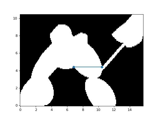
>>> from curvesimilarities.frechet import significant_events
>>> from curvesimilarities.util import parameter_space
>>> P = np.array([[0, 0], [2, 2], [4, 2], [4, 4], [2, 1], [5, 1], [7, 2]])
>>> Q = np.array([[2, 0], [1, 3], [5, 3], [5, 2], [7, 3]])
>>> events, _ = significant_events(P, Q)
>>> import matplotlib.pyplot as plt  
>>> weight, p, q, _, _ = parameter_space(P, Q, 200, 100)
>>> plt.pcolormesh(p, q, weight.T < fd(P, Q), cmap="gray")  
>>> plt.plot(*events.transpose(2, 1, 0), "o-")  

curvesimilarities.frechet.fd_matching(P, Q, param_type='arc-length', rel_tol=0.0, abs_tol=2.220446049250313e-16, event_rel_tol=0.0, event_abs_tol=2.220446049250313e-16)

Locally correct Fréchet matching [1].

A locally correct Fréchet matching is a Fréchet matching between two curves whose any sub-matching is still a Fréchet matching.

Parameters:

Pndarray

A \(p\) by \(n\) array of \(p\) vertices of a polyline in an \(n\)-dimensional space.

Qndarray

A \(q\) by \(n\) array of \(q\) vertices of a polyline in an \(n\)-dimensional space.

param_type{‘arc-length’, ‘vertex’}

Parametrization of matching.

rel_tol, abs_toldouble

Relative and absolute tolerances for parametric search of the Fréchet distance.

event_rel_tol, event_abs_toldouble

Relative and absolute tolerances to determine realizing events.

Returns:

distdouble

The (continuous) Fréchet distance between P and Q, NaN if any vertex is empty.

matchingndarray

Vertices of a locally correct Fréchet matching in parameter space.

Notes

This function implements Buchin et al.’s algorithm [1], except that backtracking is used to extract significant events.

The parametric search for the feasible distance terminates if the upper boundary a and the lower boundary b satisfy: a - b <= max(rel_tol * a, abs_tol).

An event is considered to be realizing if its value e and the realizing distnace d satisfy: e - d <= max(rel_tol * d, abs_tol).

References

[1] (1,2)

Buchin, Kevin, et al. “Locally correct Fréchet matchings.” Computational Geometry 76 (2019): 1-18.

Examples

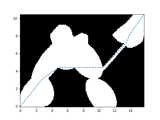
>>> from curvesimilarities.frechet import fd_matching
>>> from curvesimilarities.util import parameter_space
>>> P = np.array([[0, 0], [2, 2], [4, 2], [4, 4], [2, 1], [5, 1], [7, 2]])
>>> Q = np.array([[2, 0], [1, 3], [5, 3], [5, 2], [7, 3]])
>>> dist, path = fd_matching(P, Q)
>>> import matplotlib.pyplot as plt  
>>> weight, p, q, _, _ = parameter_space(P, Q, 200, 100)
>>> plt.pcolormesh(p, q, weight.T < dist, cmap="gray")  
>>> plt.plot(*path.T, "--")  

curvesimilarities.frechet.dfd(P, Q)

Discrete Fréchet distance between two two ordered sets of points.

Let \(\{P_0, P_1, ..., P_n\}\) and \(\{Q_0, Q_1, ..., Q_m\}\) be ordered sets of points in metric space. The discrete Fréchet distance between two sets is defined as

\[\min_{C} \max_{(i, j) \in C} \lVert P_i - Q_j \rVert,\]

where \(C\) is a nondecreasing coupling over \(\{0, ..., n\} \times \{0, ..., m\}\), starting from \((0, 0)\) and ending with \((n, m)\). \(\lVert \cdot \rVert\) is the underlying metric, which is the Euclidean metric in this function.

Parameters:

Pndarray

A \(p\) by \(n\) array of \(p\) points in an \(n\)-dimensional space.

Qndarray

A \(q\) by \(n\) array of \(q\) points in an \(n\)-dimensional space.

Returns:

distdouble

The discrete Fréchet distance between P and Q, NaN if any array of points is empty.

Notes

This function implements Eiter and Mannila’s algorithm [1].

References

[1]

Eiter, T., & Mannila, H. (1994). Computing discrete Fréchet distance.

Examples

>>> P, Q = [[0, 0], [1, 1], [2, 0]], [[0, 1], [2, -4]]
>>> dfd(np.asarray(P), np.asarray(Q))
4.0

curvesimilarities.frechet.dfd_idxs(P, Q)

Discrete Fréchet distance and its indices in curve space.

Parameters:

Pndarray

An \(p\) by \(n\) array of \(p\) points in an \(n\)-dimensional space.

Qndarray

An \(q\) by \(n\) array of \(q\) points in an \(n\)-dimensional space.

Returns:

ddouble

The discrete Fréchet distance between P and Q, NaN if any array of points is empty.

index_1int

Index of point contributing to discrete Fréchet distance in P.

index_2int

Index of point contributing to discrete Fréchet distance in Q.

Examples

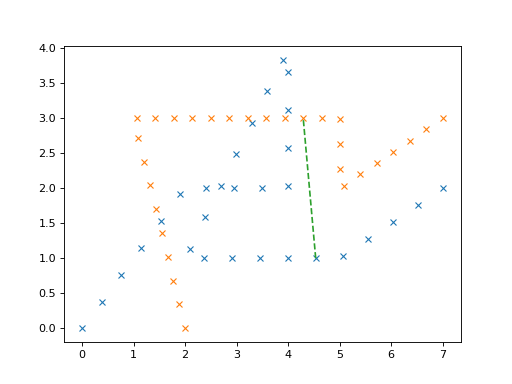
>>> P = np.array([[0, 0], [2, 2], [4, 2], [4, 4], [2, 1], [5, 1], [7, 2]])
>>> Q = np.array([[2, 0], [1, 3], [5, 3], [5, 2], [7, 3]])
>>> from curvesimilarities.util import sample_polyline
>>> P_len = np.sum(np.linalg.norm(np.diff(P, axis=0), axis=-1))
>>> P_pts = sample_polyline(P, np.linspace(0, P_len, 30))
>>> Q_len = np.sum(np.linalg.norm(np.diff(Q, axis=0), axis=-1))
>>> Q_pts = sample_polyline(Q, np.linspace(0, Q_len, 30))
>>> _, idx0, idx1 = dfd_idxs(P_pts, Q_pts)
>>> import matplotlib.pyplot as plt  
>>> plt.plot(*P_pts.T, "x"); plt.plot(*Q_pts.T, "x")  
>>> plt.plot(*np.array([P_pts[idx0], Q_pts[idx1]]).T, "--")  

Dynamic time warping distance

Dynamic time warping distance.

This module implements only the basic algorithm. If you need advanced features, use dedicated packages such as dtw-python.

curvesimilarities.dtw.dtw(P, Q, dist='euclidean')

Dynamic time warping distance between two ordered sets of points.

Let \(\{P_0, P_1, ..., P_n\}\) and \(\{Q_0, Q_1, ..., Q_m\}\) be ordered sets of points in metric space. The dynamic time warping distance between two sets is defined as

\[\min_{C} \sum_{(i, j) \in C} \lVert P_i - Q_j \rVert,\]

where \(C\) is a nondecreasing coupling over \(\{0, ..., n\} \times \{0, ..., m\}\), starting from \((0, 0)\) and ending with \((n, m)\). \(\lVert \cdot \rVert\) is the underlying metric.

Parameters:

Pndarray

A \(p\) by \(n\) array of \(p\) points in an \(n\)-dimensional space.

Qndarray

A \(q\) by \(n\) array of \(q\) points in an \(n\)-dimensional space.

dist{‘euclidean’, ‘squared_euclidean’}

Type of underlying metric. Refer to the Notes section for more information.

Returns:

double

The dynamic time warping distance between P and Q, NaN if any array of points is empty.

See also

dtw_owp

Notes

This function implements the algorithm described by Senin [1].

The following functions are available for \(\lVert \cdot \rVert\):

1. Euclidean distance

   \[\lVert p - q \rVert = \lVert p - q \rVert_2\]

2. Squared Euclidean distance

   \[\lVert p - q \rVert = \lVert p - q \rVert_2^2\]

References

[1]

Senin, P. (2008). Dynamic time warping algorithm review. Information and Computer Science Department University of Hawaii at Manoa Honolulu, USA, 855(1-23), 40.

Examples

>>> P = np.linspace([0, 0], [1, 0], 10)
>>> Q = np.linspace([0, 1], [1, 1], 20)
>>> dtw(P, Q)
20.0...

curvesimilarities.dtw.dtw_owp(P, Q, dist='euclidean')

Dynamic time warping distance and its optimal warping path.

Parameters:

Pndarray

A \(p\) by \(n\) array of \(p\) points in an \(n\)-dimensional space.

Qndarray

A \(q\) by \(n\) array of \(q\) points in an \(n\)-dimensional space.

dist{‘euclidean’, ‘squared_euclidean’}

Type of underlying metric. Refer to dtw().

Returns:

dtwdouble

The dynamic time warping distance between P and Q, NaN if any array of points is empty.

owpndarray

Indices of P and Q for optimal warping path, empty if any array of points empty.

Examples

>>> P = np.array([[0, 0], [2, 2], [4, 2], [4, 4], [2, 1], [5, 1], [7, 2]])
>>> Q = np.array([[2, 0], [1, 3], [5, 3], [5, 2], [7, 3]])
>>> _, owp = dtw_owp(P, Q)
>>> import matplotlib.pyplot as plt  
>>> x, y = np.meshgrid(np.arange(len(P)), np.arange(len(Q)))
>>> plt.plot(*np.vstack([x.ravel(), y.ravel()]), "x")  
>>> plt.plot(*owp.T, "o")  
>>> plt.axis("equal")  

Integral Fréchet distance

Integral Fréchet distance.

curvesimilarities.integfrechet.ifd(P, Q, delta, dist='euclidean')

Integral Fréchet distance between two open polygonal curves.

Let \(f, g: [0, 1] \to \Omega\) be curves defined in a metric space \(\Omega\). Let \(\alpha, \beta: [0, 1] \to [0, 1]\) be continuous non-decreasing surjections, and define \(\pi: [0, 1] \to [0, 1] \times [0, 1]\) such that \(\pi(t) = \left(\alpha(t), \beta(t)\right)\). The integral Fréchet distance between \(f\) and \(g\) is defined as

\[\inf_{\pi} \int_0^1 dist\left(\pi(t)\right) \cdot \lVert \pi'(t) \rVert_1 \mathrm{d}t,\]

where \(dist\left(\pi(t)\right)\) is a distance between \(f\left(\alpha(t)\right)\) and \(g\left(\beta(t)\right)\) and \(\lVert \cdot \rVert_1\) is the Manhattan norm.

Parameters:

Pndarray

A \(p\) by \(n\) array of \(p\) vertices of a polyline in an \(n\)-dimensional space.

Qndarray

A \(q\) by \(n\) array of \(q\) vertices of a polyline in an \(n\)-dimensional space.

deltadouble

Maximum length of edges between Steiner points. Refer to the Reference section for more information.

dist{‘euclidean’, ‘squared_euclidean’}

Type of \(dist\). Refer to the Notes section for more information.

Returns:

double

The integral Fréchet distance between P and Q, NaN if any vertice is empty or both vertices consist of a single point.

See also

ifd_owp

Notes

This function implements the algorithm of Brankovic et al [1].

The following functions are available for \(dist\):

1. Euclidean distance

   \[dist\left(p, q\right) = \lVert p - q \rVert_2\]

   Note

   This distance is not implemented yet.

2. Squared Euclidean distance

   \[dist\left(p, q\right) = \lVert p - q \rVert_2^2\]

References

[1]

Brankovic, M., et al. “(k, l)-Medians Clustering of Trajectories Using Continuous Dynamic Time Warping.” Proceedings of the 28th International Conference on Advances in Geographic Information Systems. 2020.

Examples

>>> P, Q = [[0, 0], [0.5, 0], [1, 0]], [[0, 1], [1, 1]]
>>> ifd(np.asarray(P), np.asarray(Q), 0.1, "squared_euclidean")
2.0

curvesimilarities.integfrechet.ifd_owp(P, Q, delta, dist='euclidean', param_type='arc-length')

Integral Fréchet distance and its optimal warping path.

Parameters:

Pndarray

A \(p\) by \(n\) array of \(p\) vertices of a polyline in an \(n\)-dimensional space.

Qndarray

A \(q\) by \(n\) array of \(q\) vertices of a polyline in an \(n\)-dimensional space.

deltadouble

Maximum length of edges between Steiner points. Refer to ifd().

dist{‘euclidean’, ‘squared_euclidean’}

Type of \(dist\). Refer to ifd().

param_type{‘arc-length’, ‘vertex’}

Parametrization of matching.

Returns:

ifddouble

The integral Fréchet distance between P and Q, NaN if any vertice is empty or both vertices consist of a single point.

owpndarray

Optimal warping path, empty if any vertice is empty or both vertices consist of a single point.

Examples

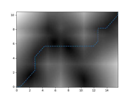
>>> from curvesimilarities.util import parameter_space
>>> P = np.array([[0, 0], [2, 2], [4, 2], [4, 4], [2, 1], [5, 1], [7, 2]])
>>> Q = np.array([[2, 0], [1, 3], [5, 3], [5, 2], [7, 3]])
>>> _, path = ifd_owp(P, Q, 0.1, "squared_euclidean")
>>> import matplotlib.pyplot as plt  
>>> weight, p, q, _, _ = parameter_space(P, Q, 200, 100)
>>> plt.pcolormesh(p, q, weight.T, cmap="gray")  
>>> plt.plot(*path.T, "--")  

Utilities

Utility functions.

curvesimilarities.util.parameter_space(P, Q, p_num, q_num)

Parameter space betwee two polylines.

Parameters:

Parray_like

A \(p\) by \(n\) array of \(p\) vertices of a polyline in an \(n\)-dimensional space.

Qarray_like

A \(q\) by \(n\) array of \(q\) vertices of a polyline in an \(n\)-dimensional space.

p_num, q_numint

Number of sample points in P and Q, respectively.

Returns:

weightndarray

A p_num by q_num array containing the distance between the points in P and Q.

p_coord, q_coordndarray

Axis coordinates for the parameter space.

p_vert, q_vertndarray

Coordinates for the vertices of polylines.

Examples

Curve space:

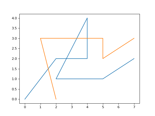
>>> P = np.array([[0, 0], [2, 2], [4, 2], [4, 4], [2, 1], [5, 1], [7, 2]])
>>> Q = np.array([[2, 0], [1, 3], [5, 3], [5, 2], [7, 3]])
>>> import matplotlib.pyplot as plt  
>>> plt.plot(*P.T)  
>>> plt.plot(*Q.T)  

Parameter space with vertices as dashed lines:

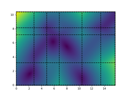
>>> weight, p, q, p_vert, q_vert = parameter_space(P, Q, 200, 100)
>>> plt.pcolormesh(p, q, weight.T)  
>>> plt.vlines(p_vert, 0, q[-1], "k", "--")  
>>> plt.hlines(q_vert, 0, p[-1], "k", "--")  

curvesimilarities.util.matching_pairs(P, Q, path, sample_num)

Sample a continuous path in parameter space to matching pairs in curve space.

Parameters:

Parray_like

A \(p\) by \(n\) array of \(p\) vertices in an \(n\)-dimensional space.

Qarray_like

A \(q\) by \(n\) array of \(q\) vertices in an \(n\)-dimensional space.

pathndarray

A \(N\) by \(2\) array of \(N\) vertices of polyline in parameter space.

sample_numint

Number of sample points to be uniformly taken from path.

Returns:

ndarray

A \(n\) by \(2\) by sample_num array of point pairs in curve space.

Examples

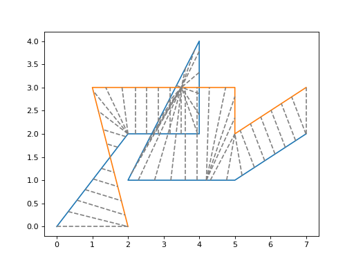
>>> from curvesimilarities import ifd_owp
>>> from curvesimilarities.util import matching_pairs
>>> P = np.array([[0, 0], [2, 2], [4, 2], [4, 4], [2, 1], [5, 1], [7, 2]])
>>> Q = np.array([[2, 0], [1, 3], [5, 3], [5, 2], [7, 3]])
>>> _, path = ifd_owp(P, Q, 0.1, "squared_euclidean")
>>> pairs = matching_pairs(P, Q, path, 50)
>>> import matplotlib.pyplot as plt  
>>> plt.plot(*P.T); plt.plot(*Q.T)  
>>> plt.plot(*pairs, "--", color="gray")  

curvesimilarities.util.sample_polyline(vert, param, param_type='arc-length')

Sample points from a polyline.

Parameters:

vertndarray

A \(p\) by \(n\) array of \(p\) vertices of a polyline in an \(n\)-dimensional space.

paramarray_like

An 1-D array of \(q\) parameters for sampled points, using arc-length parametrization.

param_type{‘arc-length’, ‘vertex’}

Parametrization type of param.

Returns:

ndarray

A \(q\) by \(n\) array of sampled points.

Glossary

arc-length parametrization

Parametrization of curve based on its arc-length. This is the default parametrization used in CurveSimilarities.

Let \(P\) be a point on a curve \(\gamma\). The parameter of \(P\) equals to the arc length of a subcurve of \(\gamma\) which begins at the starting point of \(\gamma\) and ends at \(P\).

Also known as “natural parametrization”.

vertex parametrization

Parametrization of polyline based on vertex indices and edge lengths. Useful for dealing with vertices.

Let \(P_i\) be an \(i\)-th vertex of a polyline. A point which a parameter \(t\) represents is defined as \(P_{\lfloor t \rfloor} + (t - \lfloor t \rfloor) (P_{\lfloor t \rfloor + 1} - P_{\lfloor t \rfloor})\)

matching

A matching between two curves (either continuous or discrete) \(P\) and \(Q\) is an ordered set of tuple of points \(\{(p, q) | p \in P \land q \in Q\}\).

A matching in curve space is uniquely represented by a path in parameter space.

optimal warping path

A matching determined by dynamic time warping (DTW) or integral Fréchet distance (IFD).

The term has been widely used for DTW, and we also use it for IFD since it is commonly referred to as “continuous dynamic time warping”.